

Trying It Out¶

Configuration¶

To try it out, we add a new Configuration to the routing sample that comes with OMNeT++.

Append this section to the omnetpp.ini file in the samples/routing directory:

[Config MeshExperiment]
network = networks.Mesh
**.width = ${10..20 step 2}
**.height = ${10..20 step 2}

**.destAddresses = "0 2 5 6 9 14 17 18 23 27 29 36 42 52 89 123 150 183 192"
**.sendIaTime = uniform(100us, 10ms)  # high traffic

**.vector-recording = false
sim-time-limit = 10s

This configuration tries to make each of its runs execute for a significant amount of time - about a minute each on average - by setting up a large network with a small packet inter-arrival time and a relatively long simulation time limit. It also disables vector recording to keep the size of the result files within the limits of the presented solution.

Execution¶

To run it, open a terminal, set up the necessary environment variables using setenv, then change into the directory of the sample:

$ cd /path/to/omnetpp/
$ . setenv
$ cd samples/routing

Then execute the client.py script, substituting the IP address of your Redis server on AWS:

$ python3 /path/to/client.py ./routing -c MeshExperiment --redis-host 172.17.1.19

You should see all runs submitted to the job queue, and after a while, finishing them. The results should appear in the results directory, just like with local execution.

Comparison¶

You can compare the performance of the cloud solution with that of your own machine by running the same campaign on both, through the time utility:

$ time python3 /path/to/client.py ./routing -c MeshExperiment --redis-host 172.17.1.19
    …
$ time opp_runall ./routing -c MeshExperiment

After the output of each command, time will print a summary of the execution times.

Locally on my computer, using all 8 of its cores, the times were:

real    4m37.610s
user    25m4.576s
sys 0m0.870s

The most interesting from our perspective is the real time, as this shows the amount of wall-clock time it took to run each command. The user time is the net processing time. It is much more than the real time, because it is aggregated across all cores.

And of the one running on AWS:

real    4m12.310s
user    0m1.931s
sys 0m1.925s

With just 3 single-core workers, the simulation completes faster than running on 8 local cores. The user time is next to negligible in this case, because my computer spent most of the time idling, waiting for the results to come back.

Shutting Down¶

To prevent the aimless and useless exhaustion of your Free Tier resource allowance (or in the long term, your credit card balance), it is important to terminate your allocated resources once you are done using them. In our case, these are the EC2 Instances started by the ECS Cluster. We need to shut these down, because when calculating their usage, the whole amount of time the instances are running (or paused, but kept available) is taken into account, not just the time when they were actually used, doing something useful.

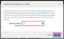
If you wish to use the Cluster again later, the easiest thing to do is scaling down the number of underlying EC2 Instances to 0. This will of course cause all running tasks to stop, as they no longer have anything to run on.

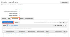
Alternatively, you can delete the whole Cluster. This will also terminate the EC2 Instances, but it will delete the worker Service as well.

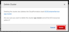
The Task Definitions are not deleted either way, but this is not a problem, since they can be kept around indefinitely, free of charge.