Part 5 - Adding Statistics Collection
5.1 Displaying the number of packets sent/received
To get an overview at runtime how many messages each node sent or received, we've added two counters to the module class: numSent and numReceived.
They are set to zero and WATCH'ed in the initialize() method. Now we
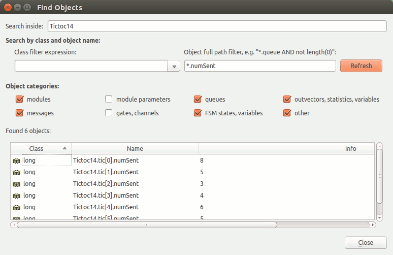
can use the Find/inspect objects dialog (Inspect menu; it is also on
the toolbar) to learn how many packets were sent or received by the
various nodes.
It's true that in this concrete simulation model the numbers will be
roughly the same, so you can only learn from them that intuniform()
works properly. But in real-life simulations it can be very useful that
you can quickly get an overview about the state of various nodes in the
model.
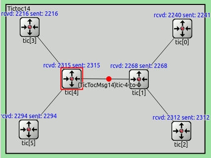
It can be also arranged that this info appears above the module
icons. The t= display string tag specifies the text;
we only need to modify the displays string during runtime.
The following code does the job:
And the result looks like this:
5.2 Adding statistics collection
The previous simulation model does something interesting enough so that we can collect some statistics. For example, you may be interested in the average hop count a message has to travel before reaching its destination.
We'll record in the hop count of every message upon arrival into an output vector (a sequence of (time,value) pairs, sort of a time series). We also calculate mean, standard deviation, minimum, maximum values per node, and write them into a file at the end of the simulation. Then we'll use tools from the OMNeT++ IDE to analyse the output files.
For that, we add an output vector object (which will record the data into
Tictoc15-#0.vec) and a histogram object (which also calculates mean, etc)
to the class.
When a message arrives at the destination node, we update the statistics.
The following code has been added to handleMessage():
The hopCountVector.record() call writes the data into Tictoc15-#0.vec.
With a large simulation model or long execution time, the Tictoc15-#0.vec file
may grow very large. To handle this situation, you can specifically
disable/enable vector in omnetpp.ini, and you can also specify
a simulation time interval in which you're interested
(data recorded outside this interval will be discarded.)
When you begin a new simulation, the existing Tictoc15-#0.vec/sca
files get deleted.
Scalar data (collected by the histogram object in this simulation)
have to be recorded manually, in the finish() function.
finish() is invoked on successful completion of the simulation,
i.e. not when it's stopped with an error. The recordScalar() calls
in the code below write into the Tictoc15-#0.sca file.
The files are stored in the results/ subdirectory.
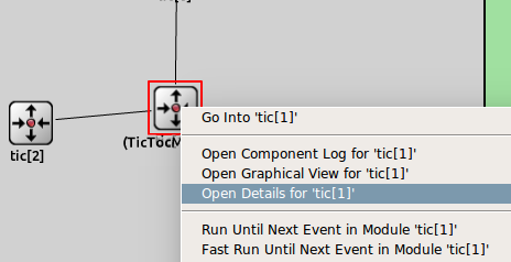
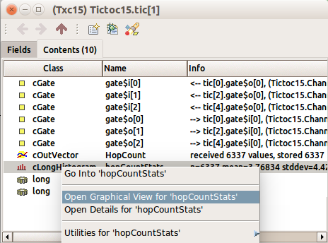
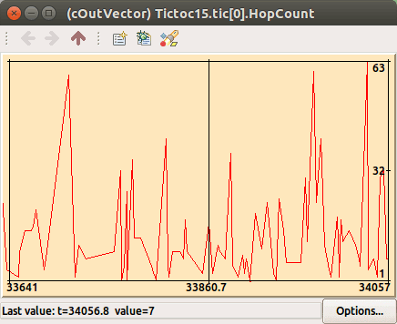
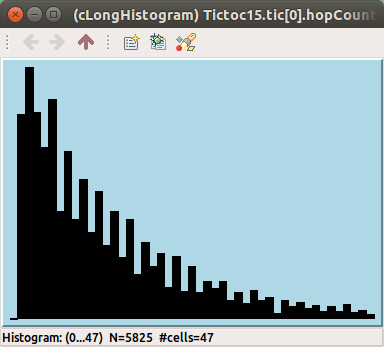
You can also view the data during simulation. To do that, right click on a module, and
choose Open Details. In the module inspector's Contents page you'll find the hopCountStats
and hopCountVector objects. To open their inspectors, right click on cHistogram hopCountStats or
cOutVector HopCount, and click Open Graphical View.
The inspector:
They will be initially empty -- run the simulation in Fast (or even Express) mode to get enough data to be displayed. After a while you'll get something like this:
When you think enough data has been collected, you can stop the simulation
and then we'll analyse the result files (Tictoc15-#0.vec and
Tictoc15-#0.sca) off-line. You'll need to choose Simulate -> Call finish()
from the menu (or click the corresponding toolbar button) before exiting --
this will cause the finish() functions to run and data to be written into
Tictoc15-#0.sca.
5.3 Statistic collection without modifying your model
In the previous step we have added statistic collection to our model. While we can compute and save any value we wish, usually it is not known at the time of writing the model, what data the enduser will need.
OMNeT++ provides an additional mechanism to record values and events. Any model can emit signals that can carry a value or an object. The model writer just have to decide what signals to emit, what data to attach to them and when to emit them. The enduser can attach 'listeners' to these signals that can process or record these data items. This way the model code does not have to contain any code that is specific to the statistics collection and the enduser can freely add additional statistics without even looking into the C++ code.
We will re-write the statistic collection introduced in the last step to
use signals. First of all, we can safely remove all statistic related variables
from our module. There is no need for the cOutVector and
cHistogram classes either. We will need only a single signal
that carries the hopCount of the message at the time of message
arrival at the destination.
First we need to define our signal. The arrivalSignal is just an
identifier that can be used later to easily refer to our signal.
We must register all signals before using them. The best place to do this
is the initialize() method of the module.
Now we can emit our signal, when the message has arrived to the destination node.
As we do not have to save or store anything manually, the finish() method
can be deleted. We no longer need it.
The last step is that we have to define the emitted signal also in the NED file. Declaring signals in the NED file allows you to have all information about your module in one place. You will see the parameters it takes, its input and output gates, and also the signals and statistics it provides.
Now we can define also a statistic that should be collected by default. Our previous example has collected statistics (max, min, mean, count, etc.) about the hop count of the arriving messages, so let's collect the same data here, too.
The source key specifies the signal we want our statistic to attach to.
The record key can be used to tell what should be done with the received
data. In our case we specify that each value must be saved in a vector file (vector)
and also we need to calculate min,max,mean,count etc. (stats). (NOTE: stats is
just a shorthand for min, max, mean, sum, count, etc.) With this step we have finished
our model.
Now we have just realized that we would like to see a histogram of the hopCount on the
tic[1] module. On the other hand we are short on disk storage and we are not interested
having the vector data for the first three module tic 0,1,2. No problem. We can add our
histogram and remove the unneeded vector recording without even touching the C++ or NED
files. Just open the INI file and modify the statistic recording:
We can configure a wide range of statistics without even looking into the C++ code, provided that the original model emits the necessary signals for us.
5.4 Adding figures
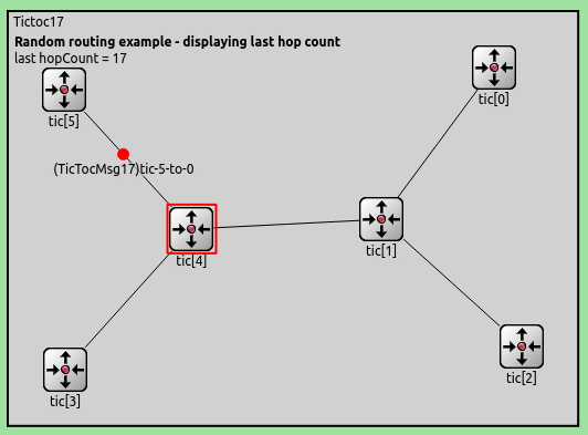
OMNeT++ can display figures on the canvas, such as text, geometric shapes or images. These figures can be static, or change dynamically according to what happens in the simulation. In this case, we will display a static descriptive text, and a dynamic text showing the hop count of the last message that arrived at its destination.
We create figures in , with the @figure property.
This creates two text figures named description and lasthopcount, and sets their positions on the canvas (we place them in the top right corner).
The font attribute sets the figure text's font. It has three parameters: typeface, size, style. Any one of them
can be omitted to leave the parameter at default. Here we set the description figure's font to bold.
By default the text in lasthopcount is static, but we'll
change it when a message arrives. This is done in , in the handleMessage() function.
The figure is represented by the cTextFigure C++ class. There are several figure types,
all of them are subclassed from the cFigure base class.
We insert the code responsible for updating the figure text after we retreive the hopcount variable.
We want to draw the figures on the network's canvas. The getParentModule() function returns the parent of the node, ie. the network.
Then the getCanvas() function returns the network's canvas, and getFigure() gets the figure by name.
Then, we update the figure's text with the setText() function.
Tip
For more information on figures and the canvas, see The Canvas section of the OMNeT++ manual
When you run the simulation, the figure displays 'last hopCount: N/A' before the arrival of the first message. Then, it is updated whenever a message arrives at its destination.
Tip
If the figure text and nodes overlap, press 're-layout'.

In the last few steps, we have collected and displayed statistics. In the next part, we'll see and analyze them in the IDE.